Estimating Vehicle Parameters with Constrained Optimisation

While complementary sensors provide useful data, it is not always obvious how to use this information to improve our estimation of a vehicle's characteristics. We are currently investigating constrained optimisation techniques that use complementary sensor data to reduce the ambiguity of this estimation. We will first describe optimisation in the context of iBWIM and then describe how additional information, for example the vehicle's class, can improve our estimate of the vehicle's parameters.

Analytical Methods and Optimisation Methods for iBWIM

The Analytical Method

The standard method for estimating vehicle parameters is an analytical approach. A set of equations is derived that use vehicle parameters to predict the strain signal. We call this the forward model. This equation set is inverted and solved—this is the inverse model. We can simply slot our measured strain signal into the inverse model and recover the axle pattern and loadings. The calculation is direct; there is a single, unambiguous solution.

This approach rests on a number of assumptions which may be more or less valid depending on the properties of the bridge. When these assumptions break down, the analytical approach may not be robust, i.e. a small error in the model or the measurement may give rise to an estimate that is entirely wrong. Unfortunately, because the calculation is essentially a black box to the user, there is no way to correct or "steer" the estimate to more plausible values. Nor is it easy to incorporate information from outside the analytical model, for instance from complementary measurement systems or from plausibility constraints. Optimisation techniques are one way of incorporating additional sources of information and of avoiding the "brittleness" associated with an inversion model.

Optimisation for iBWIM

Optimisation approaches define a hypothetical vehicle, with initial guess about its axle loadings and pattern. The forward model is used to predict what strain signal would be produced by this vehicle. This prediction is compared with the measured signal and the difference between the two, the error value, is measured. Depending on the error term the vehicle model is adjusted to produce a prediction that fits the measurement more closely. This process of comparison and adjustment is repeated iteratively, until step by step the prediction converges with the measured signal. At this point, we assume that our model of the vehicle accurately represents the real vehicle.

What does the optimisation process look like?

The measured strain signal consists of a series of overlapping peaks—with each peak corresponding to one of the vehicle's axles. In our model we approximate each of these peaks as a Gaussian parameterised by amplitude, mean and standard deviation. Amplitude corresponds to the axle's loading, mean to its location (relative to the other axles), and standard deviation is a function of the dynamic characteristics of vehicle and the bridge. We vary the parameters of each Gaussians (shown in isolation in the lower graph) and approximate the strain strain signal with the sum of these Gaussians (top graph). The error term is the difference between the measurement and the prediction. As the estimate improves, the error term converges to zero.

What is happening when we optimise?

We can gain more insight into the process by plotting the error as a function of the parameters we are trying estimate. To allow visualisation we limit ourselves to two parameters: the loadings of the second and third axles. In reality, we would be estimating something of the order of twenty parameters. To make the graph clearer we plot -1 times the error term—this means we are asking the algorithm to find the maxima of the error function. The algorithm's task is analogous to finding the highest point in a landscape, without a map and in the dark.

The landscape shown opposite illustrates two of the difficulties an optimisation algorithm may face. The first is that there are multiple local maxima, i.e. there are three hills each of which has a summit that is highest point in its neighbourhood. Although a summit may be the highest point in its own locality it might not be the highest point in the landscape. In our application that means that there may be several vehicle models that can explain the strain signal reasonably well, though only one resembles the actual vehicle characteristics. The traditional method for dealing with this problem is to run the algorithm several times with different initial guesses, then to select the best overall solution.

The second issue is connected with the ridge on which the global maxima lies. When a solution lies in a region, or a curve, where the error function is flat then varying one or more parameters may not have a dramatic effect on the quality of the fit—even if it radically changes the characteristics of the vehicle model. If this is the case, small measurement or model errors may result in us settling on a vehicle model that is radically wrong. In practice, both this problem, and the problem of local sub-optimal solutions are not unique to the optimisation approach. They are, after all, implicit in the physical system—it is just that they are more obvious is the explicit calculations carried out during optimisation.

Using new data with optimisation

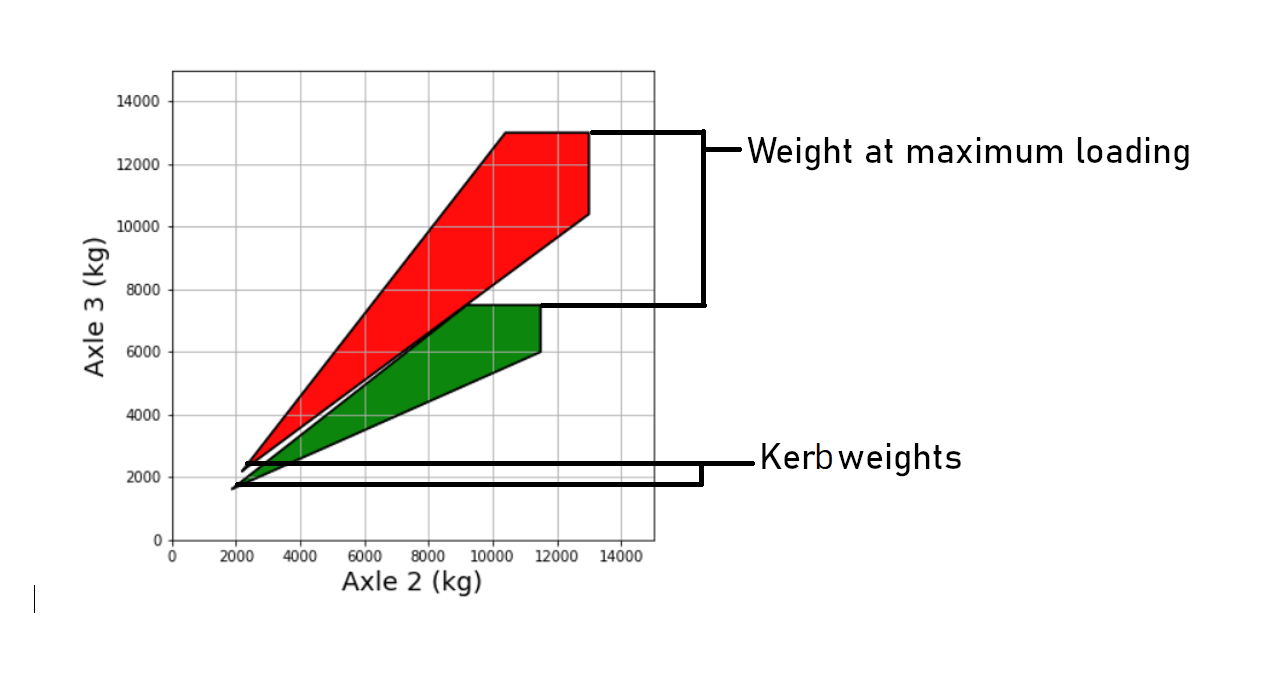
One of the advantages of optimisation is that it allows us an easy way to introduce new information, either in the form of common sense or from complementary sensors. For instance, our complementary sensors might tell us that we are dealing with a Mercedes 3 axle tractor unit for a semi-trailer. With this information we can constrain the estimates of axle weights to the trapezoid discussed in the fig 1. We can, firstly limit our initial guesses for these parameters to be within the trapezoid and secondly, we can modify the penalty function to discourage solutions outside this area.

Summary<

This is obviously a simplified example, we are optimising only two parameters, when a more realistic number would be twenty. However, in reality we would able to make very good initial guesses from simple peak finding in the strain signal. Together with constraints about plausible axle patterns and loadings, this will dramatically reduce the search space that must be optimised. This means computation is reduced and it is feasible to conduct the optimisation in real-time.