iBWIM measures vehicle parameters—it is natural to use this data to classify vehicles by type. iBWIM has always done so, either using the broad classes set out in COST323, or into much more specific categories required by some of our clients. A description of some important classification schemes is given here. We are currently working on a number of technologies to provide an even finer grain classification.
A highly specific vehicle classifier has two advantages:
The simplest way to discriminate between vehicle categories is axle count. This is the first (simplifying) step in all our algorithms. The next obvious feature is the axle groupings: i.e. how are the axles spaced? are they grouped in pairs or triples? With a simple set of IF THEN rules we can discriminate many classes of vehicle based on their axle distances. Figure 1 shows a plot of the distances between the first and second, and second and third axles for three axle vehicles. Simple rules will discriminate many, though not all of the classes shown.
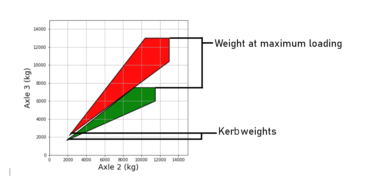
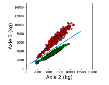
Consider a simple case where we wish to discriminate a Mercedes Acros 3 axle semi-trailer from its tipper variant. The unloaded and fully loaded axle weights are specified be the manufacturer, we can plot the possible loadings of these two axles on a two dimensional plot, Figure 2. The unloaded (kerb) weight is the lower vertex on the diagonal of trapezoid; the maximum loading is the upper vertex. The adjacent vertices allow for natural variation in the measurements. If we were to measure a set of vehicles belonging to these two classes, with various loads, and plot their second and third axle loadings we would get a distribution of the form shown in Figure 3. Simply using one axle load would not be enough to tell us to which class a given truck belongs; however, with both axle loadings and a simple rule (blue line), we can confidently discriminate between the tipper and the semi-trailer.